1. Basic Themes in Excel

Zen and the Art of Excel Spreadsheeting...
In Excel, the most elegant solution is always the simplest. Teach Excel with love and care, and your students will recognise how much effort they can conserve! Teach them the path of least resistance. Teach them that mastery of this package requires diligence, discipline and dedication, just like the noble art of Zen. Or Origami. Or anything silly and vaguely oriental-sounding. It makes them laugh, and breaks the ice over what, for many, is a nerve-wracking experience, as they equate Excel with maths and 'all that scary stuff' they were 'rubbish at' at school.

Navigation, layout and fundamentals

You will, of course, have asked a quick relay question at the beginning of the first class, to establish extent of current knowledge. This will dictate how quickly or slowly you cover the basics. You will still get learners turning up who have never used an application so don't ever underestimate the use of this section.

As with the other applications, I will always take a top-down guided tour of the screen:
Long blue bar across the top, running from left to right, this is the title bar - tells us we're in Microsoft Excel, and that we're in 'Book1'. Question - why 'book1', and not, say, 'file1', or 'spreadsheet1', or something? A: - because it's got pages in it - i.e. sheets (draw their attention to the tabs at the bottom). Although spreadsheet is a generic term, the one Microsoft uses is Workbook, and in it are Worksheets. Hence the generic names of Book1 and Sheet1. These terms are used readily in the Help files but aren't actually defined!

Underneath the Title Bar are the drop-down menus, followed by the toolbars. Trick: Sometimes, especially versions 2002 and 2003, the two basic toolbars (Standard and Formatting) are squashed onto one row, and the drop-downs only show the most-used features. Get them to sort this out now - easiest way is Tools->Customise; Options tab; choose the options for Show Standard and Formatting on two rows and Always show full menus. Much better.

Familiarise learners with the Name Box (used for identification, navigation and also for Named Ranges, but don't introduce this last concept at this stage); with the Formula Bar and with the spreadsheet itself, in particular cells, columns and rows.

What happens when we get to column Z? What's the next column along called? (Encourages exploration and use of the horizontal scroll bar.) What's the final column called? (A: IV) How many columns do you think this is altogether? (A: 256). So how many rows do we have? ... If anyone's scrolling down, stop now - we have 65,536 altogether! So - does anyone know their 256 times table? No? ;-) We have close on to 17 million cells in this one sheet alone. Add in the others, and we have a lot of space to play with - don't think that you're ever going to run out of space, it's not likely to happen! (But do note that advanced users have done just this, loads of times - hence version 2007 giving us 1,048,576 rows by 16,384 columns, with the columns now ending at XFD instead of IV. If students consistently need more, they would be better off using Access or another databasing package.)

Cover selecting cells, rows, columns and the whole spreadsheet (include selecting non-contiguous cells for the more advanced classes). Cover navigation both by mouse and keyboard - draw attention to the need to confirm by using [Enter] in Excel and reinforce this at every opportunity - try and get out of the habit of 'clicking out' of the cell as you will cause yourself a lot of problems later on, especially when we come to formulae.

Follow the instructions in the Status bar - it helps new users a lot. Firstly a cell will have a status of 'ready'. When we start to type it says 'Enter' (so it's telling us to press the Enter key). If we go back to edit a cell, it says 'Edit'. There are various other helpful messages down there.

Cover using Autofill to create lists of days, months, dates, numbers and other series. Don't forget to show that Autofill can be used to the right as well as down. Overview widening columns and Autofit.

Creating and modifying spreadsheets

Like Word, Excel has four processes which newbies need to familiarise themselves with - creating a new spreadsheet, opening an existing one, saving a spreadsheet, and closing it. You may need to embed some file management principles here - navigating around the Open or Save dialog boxes, the difference between Save and Save As, etc. Be prepared to be patient as lots of people are unaware of these basics. Give plenty of opportunity to practise, and be ready with your 1:1 support.

Good spreadsheets should always have two things: labels and data. A label is info that tells you what you're looking at - column or row headings. Data is stuff in the spreadsheet itself - people's names, items in a stocklist, prices, phone numbers - anything.

It's important to have both of these elements. Sure you can have a spreadsheet without data, but data without labels is really daft. You will think you'll remember what the data is, three months down the line when you come to open it again, but you really won't, and you'll be left wondering what the heck you were thinking of when you created it!

Modifying is often 'unintuitive' (extuitive?) for beginners. They feel they have to remove the existing value before typing in new information, or that they have to click into the cell (into 'edit' mode) and select the value before formatting. This is when using the term 'active cell' can be handy, because if you say "all you have to do is make sure your active cell is the one you want to modify, and away you go", then there is no emphasis on 'clicking into' the cell or doing anything at all to the cell's contents. If they prefer keyboard to edit, draw their attention to F2.

Copying/moving data/rows/columns

Duh, this is not obvious, believe me. It's really not the same as Word. For a start, when you cut in Word, the text disappears. In Excel, it stays there, with a merry dotted line running round the edge. And it doesn't matter if you cut or delete in Word, the effect is the same - the text disappears. In Excel, cut and delete do very different things.

Having said that, it's a pretty simple process for the learners to get to grips with, so spend no more than 15-30 minutes on it.

I have learnt from experience that the easiest and most consistent way is to advocate use of the right-click menu, as cut, copy, paste, delete and insert are all there. The best way to practise is on a spreadsheet with data in - if you're worried they will lose valuable data, get them to do a Save As or have a dedicated cuttypasty exercise.

Start with deleting entire columns or rows. Note how the column isn't deleted, but the data's 'slid across' - we still have the same number of columns.

Move onto inserting entire columns or rows. Which column will I need to select, the one to the left or the one to the right? Students will volunteer suggestions, so let them try whichever they want. If it's the wrong one, what can I do? Undo! It will take a bit of practice, but if you remember you always have Undo to bail you out, you can't go too far wrong.

Then move onto inserting/deleting individual cells. Start off with 'shift cells right' then go for 'shift cells down'. Try it within a spreadsheet with formulae in, so they can see how the formula adjusts to take account of its new location (this can be a great intro to relative cell referencing). Once they've done that, they can try deleting with 'shift cells up' or 'shift cells left'. You can also introduce them to the concept of inserting/deleting a range at this stage, if they're particularly switched on.

As for cutting and copying, try to explain the difference between cutting and inserting, and cutting and pasting. It can help if you have a spreadsheet with numbered data on it. Ask them to select an entire row or column (as before, it's a lot easier to demonstrate entire rows/columns), then right-click and cut. Choose a new location and ask them what they think the difference will be between 'paste' and 'insert cut cells'. (Basically, cut and paste takes from the old location and sticks it straight onto the top of the new location - including over any existing data. Cut and insert takes from the old location, and tucks it into the new location, between the data.) Ask them to right-click and cut from the same original row, and if you tried right-click-insert last time, try right-click-paste this time. They can then compare the difference.

It's a simple process then to show them the way copy (with paste, or with insert copied cells) works.

Trick: if you want to be rid of the dotted border after cutting or copying, press the Esc key on the keyboard.

Printing, print preview, page setup and layout

Oh my word, what fun and games you can have if you don't know your way around Excel's printing options. Trick: unplug the printer now, please, unless you're going to charge your students per tree of paper they use by mistake. And clear the print queue before you plug it back in!

The main reason to teach printing in Excel is simply because the information isn't contained, neatly, on pages, like it is already in Word. You can always label this section 'advanced printing' if you think your learners will be patronised by a section on 'printing' alone. I'm really of the opinion that there's so much going on with printing in Excel that it should even have its own drop-down menu.

It's up to you what kind of data is on your 'base' spreadsheet, but something that goes down or over a few pages (if you were to print it out, that is) will be handy for them to understand some of the things you show them.

Random statistic: If you were to print the whole of one worksheet, you'd use 36,000 sheets of paper - a stack about 6 feet tall. Eeep!

1. Always look at your spreadsheet via Print Preview first.

   Advise them that nothing in these options actually changes the spreadsheet, we're only tinkering with the printed output.

   Start off by demonstrating the 'Zoom' tool -the magnifying glass that allows you to 'bring the paper forward' or 'push it away again' just by clicking in the middle of the 'paper'.
    

2. Work through the four tabs in the Setup dialog box.

   You may need to do a quick demo here, as some learners will not have come across a dialog box with tabs before, so they need to know what you're talking about. There are quite a few in Excel, too, so they need to be familiar with them.

   You must ensure that learners don't close the Print Preview, as then they can't see the effects of their changes.

   Page tab: Orientation: obvious. Scaling: I use this for shrinking or enlarging the output so it fits all on one page. Click OK to return to the preview to check how it looks.

   Margins tab: Useful only really to set centring horizontally and vertically. For this, I usually return to the preview screen and use the Margins button at the top. Trick: Advise that the 'tags' that connect from top to bottom and left to right are the only ones that should be moved, these change the margins (and can be very handy to fix those times when a single column falls onto a new page all by itself). DON'T touch the unconnected tags at the top, as you will actually be affecting your spreadsheet, and there's NO undo!!

   Header/Footer tab: Ooh, this can be fun.
   Click on the Custom Header button, and you will find three panels, corresponding to the areas on the page.
   Walk the learners through each of the buttons in turn, on the mini-toolbar that's part of the dialog box:
     

   Start by typing your name in the left-hand panel, then to format it, select the text and choose the first button in the toolbar, the A button. You don't get many choices, but hey, this isn't really the important part of your document! In the centre panel, show them how to use the next two buttons. DEMO THIS PART, I can't stress this enough, people just won't get it otherwise.

   Clicking will give you the code &[Page], which will automatically tell you what page you're on. Clicking gives you &[Pages], which will say how many pages in total there are. It is important not to mess around with this code, otherwise Excel won't be able to do what you ask it to.   If you just click on the first button then the second, you end up with the code &[Page]&[Pages] which is liable to return the text '11' (the first 1 because it's viewing page 1, and the second 1 because there is 1 page in total). You need to pad it out with typed-out text in order for it to make sense:   Here, the red bits are the code, and the blue bits are the extra text which you type yourself:  Page &[Page] of &[Pages] (don't forget the spaces)   which will end up as the more logical Page 1 of 1 on your preview.   In the right-hand panel, get them to experiment with the next few buttons, which return code of &[Date], &[Time], &[Path]&[File](i.e. where you've saved it as well as the file name), &[File] or &[Tab].   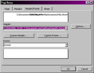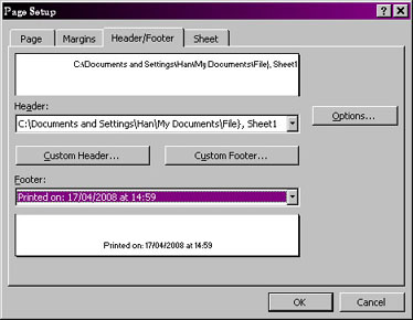Do note that sometimes the text end ups very long and actually overlaps onto other text, as you can see on the left image. Solution: split the information into the footer, as seen on the right.      Don't bother with the picture option, unless you have a very small pic, like a logo or something.

   Sheet tab: This last tab is handy.
   Print area and Print titles will be greyed out for now - see below for info on this.
   Print: gridlines - very handy! Makes spreadsheets a lot more readable; Black and white is obvious; Draft quality is a low-ink version if you're printing out at home but note that it cancels out the Gridlines setting and they won't print; Row and Column headings is also handy but not so obvious to newbies so get them to try it anyway; Cell errors - if you want to have your #VALUE or whatever displayed. Comments will also be greyed out for now - see below for info.
   Page order: I tend not to worry about this!
    

3. Further print options/problems can be caused by the stupidity of the way all the print options are scattered throughout the program. I use this with intermediate users, and it's handy as a time-filler.
   Trick: make sure you are NOT in Print Preview for these options, they will NOT work.

Printing the same information at the top or side of each page: This is known as Print Titles. File -> Page Setup Sheet tab, Print titles section Click in the Rows to repeat at top panel Click back on your spreadsheet somewhere in Row 1 (or click and drag for more than one row) Repeat for columns, if necessary Click OK.

Printing comments: Show the comment in the spreadsheet and reposition as preferred File -> Page Setup Sheet tab, Print section Choose which option from the Comments drop-down you want - None, At end of sheet, or As displayed on sheet Click OK. Note: if you want to see what this looks like, you can go for Print Preview and will now see your choice there.

Page break preview: This view is used to see how your spreadsheet has been split into different pages by Excel. View -> Page break preview OR Print Preview -> Page break preview button To amend the extent of individual pages: Hover over the blue lines, and click and drag up/down or left/right. Dotted lines indicate page breaks that Excel has put in, rather than where you chose them to be. Your spreadsheet is still editable in this view. You can increase the size of it by using your Zoom button on the Standard toolbar. To return to the normal view, go to View -> Normal.

Setting the Print Area: This is useful if you have a large spreadsheet and only need to print out a small area each time. Select the range of cells you want to set as a print area. File -> Print Area -> Set Print Area To change your mind, head to File -> Print Area -> Clear Print Area.

One last note: Whenever you first play around with print options in Excel, it will place, on your spreadsheet, dotted lines around each page. There are two ways of clearing this: a) Tools-> Options, View tab: Uncheck the option for Page Breaks; b) saving, closing and reopening!

I hope this demonstrates that using printing in Excel is not child's play!

Head off to page 2 - using formulae in Excel.